Solver-agnostic core

axqua.core contains everything that describes the free-surface water body and the modeling task independently of a simulation code. No module of this package imports a backend.

Geodata and rasters

One reader for a case’s geodata layers.

Before this module, every part of axqua that needed a layer opened it itself: fourteen modules each doing their own gpd.read_file plus a CRS reprojection, with no caching. _read_mesh_zones alone was called from five places in a single build, re-reading the same GeoPackage every time, and two modules reached into another module’s private _channel_union because there was nowhere shared to put it. This is that shared place.

What is cached, and what deliberately is not

Only the raw layer is cached - the expensive part, the disk read and the reprojection. Everything derived from it is recomputed per call, because derived values depend on configuration that legitimately changes during a session: the mesh-convergence study rebuilds the same case at a ladder of mesh.size_scale values, and caching the scaled zone edge lengths would hand every level after the first the sizes of the level before it. That is a silent wrong-answer bug rather than a crash, so the split is enforced by construction: Dataset.mesh_zones() derives its columns fresh each time from a cached frame.

Layer sources

A layer may be given as a path (the normal case) or handed over already loaded via Dataset.set_layer(). The second form exists because a QGIS plugin has the layers open in the project already, and forcing it to write temporary GeoPackages so axqua can read them back would be absurd.

axqua.core.geodata.match_field(gdf, name)

Case-insensitive column lookup (so ‘Zone Name’/’zone name’ both match).

Parameters:

name (str)

Return type:

str | None

axqua.core.geodata.parse_decimal(value)

Parse a numeric attribute robustly.

A GeoPackage double field already comes back as a float, but a field authored in a German-locale GIS may arrive as the string "0,5". Accept both: floats/ints pass through; strings have their decimal comma normalized to a point before parsing. Returns None for blanks / NaN / unparseable values so the caller can fall back to a configured default.

Return type:

float | None

axqua.core.geodata.classify_zone(name)

Map a ‘Zone Name’ to a zone type by substring (case-insensitive).

Parameters:

name (str)

Return type:

str

axqua.core.geodata.fill_holes(geom)

Return geom with all interior rings removed (only the exterior kept).

A mesh-zone author commonly carves holes into the channel polygon so a finer refinement zone can be nested inside (e.g. around a structure). Such a hole is enclosed by channel on every side, so it is channel - just meshed finer. Dropping the holes keeps those nested pockets part of the channel footprint so they are pre-wetted with the rest of the channel.

class axqua.core.geodata.Dataset(cfg)

Bases: object

A case’s geodata layers, read once and reprojected to the project CRS.

set_layer(role, frame)

Supply a layer directly instead of reading it from disk.

The seam a QGIS plugin needs: it already has the layers open, and should not have to round-trip them through temporary files. Also useful in tests.

Parameters:

role (str)

Return type:

None

layer(role, path=None)

The raw layer for role, read at most once per Dataset.

Only this - the disk read and the reprojection - is cached. Anything derived from a layer is recomputed by its caller, because it may depend on config that changes between calls (see the module docstring).

Parameters:

role (str)

has(role, path=None)

Parameters:

role (str)

Return type:

bool

roi_polygon()

The region of interest as a shapely Polygon (polygonising lines if needed).

mesh_zones()

Mesh-zone polygons with the derived columns the meshers need.

Adds, per polygon:

• _zone_type - channel / floodplain / refinement / other, from the Zone Name field (classify_zone());

• _edge_length - target max edge length [m] from the Max Edge Length (m) field (mesh.zone_size_field), falling back to the configured per-type default, then multiplied by mesh.size_scale;

• _prio - overlap priority, finest intent winning.

Recomputed on every call, never cached: mesh.size_scale is varied by the convergence study between builds of the same case, and a cached _edge_length would give every level the previous level’s sizes.

channel_union()

Channel footprint: union of the *channel* mesh zones, holes filled.

Cacheable despite deriving from mesh_zones(), because it uses only _zone_type and the geometry - neither of which mesh.size_scale touches.

centerline()

The channel centerline as a single merged LineString (longest part).

centerline_tangents(spacing)

Sample the centerline -> (points, unit tangents, KD-tree).

Cached per spacing: the anisotropic mesher and the pre-wetting ask for different samplings of the same line, and each is a few thousand interpolate calls.

Parameters:

spacing (float)

roughness_zones()

roughness_table()

{zone_id: roughness} from the zone-roughness CSV.

The first column is the integer zone id, the second the roughness value (e.g. a Nikuradse k_s) that HydroBayesCal later adjusts. A header row is detected and skipped; further columns are ignored.

Return type:

dict[int, float]

lines(role, path)

Coordinate lists of every line in a layer (breaklines, and similar).

Parameters:

role (str)

region_seeds()

(xy, matid) of the region seed points, or (None, None).

liquid_boundaries()

The raw inflow/outflow (and internal) boundary-line layer.

One of the most re-read layers in the codebase: the steering writer, the boundary classifier, the water-table fit and both meshers all want it, and each used to open it again.

structures()

The raw dam / weir / wall / building layer.

centerline_frame()

The raw centerline layer (callers that want the geometries, not tangents).

class axqua.core.geodata.ZoneRoughness(zone_id, ks, ks_min=None, ks_max=None, calibrate=None)

Bases: object

One row of the zone-roughness CSV.

ks is the nominal roughness that seeds the friction .tbl and the geometry’s BOTTOM FRICTION; for a calibrated zone the calibrator overwrites it on every run, so it only has to be a sane starting point. ks_min / ks_max are the calibration prior bounds and calibrate says whether the zone is a calibration parameter at all (None = the table does not say, so the decision falls back to the config’s parameter list).

Parameters:

• zone_id (int)

• ks (float)

• ks_min (float | None)

• ks_max (float | None)

• calibrate (bool | None)

zone_id: int

ks: float

ks_min: float | None = None

ks_max: float | None = None

calibrate: bool | None = None

axqua.core.geodata.read_roughness_zones(path)

Standalone reader for the zone-roughness CSV (no Dataset required).

Two schemas are accepted, distinguished by the header:

• bounds - zone_id, ks_min, ks_max[, calibration]: the nominal ks is the midpoint of the prior, matching how a uniform prior’s central value is chosen elsewhere. A zone whose bounds are equal is a fixed roughness.

• legacy - zone_id, ks: one value per zone, no bounds, no flag.

Header names are matched case-insensitively after stripping whitespace (the hand-edited CSVs carry , ks_max with a leading space), and a headerless file falls back to positional columns.

Return type:

dict[int, ZoneRoughness]

axqua.core.geodata.read_roughness_table(path)

Standalone reader for the zone-roughness CSV -> {zone_id: nominal ks}.

The nominal value seeds the friction .tbl and the geometry’s BOTTOM FRICTION; see read_roughness_zones() for the full record (prior bounds + calibration flag).

Return type:

dict[int, float]

axqua.core.geodata.nominal_channel_size(cfg)

Effective (scaled) target channel edge length [m].

The smallest channel-zone _edge_length from the mesh-zones gpkg when configured (per-zone Max Edge Length (m) values override the *_size fallbacks, so channel_size alone can misstate the built resolution), else channel_size * size_scale. Both already include mesh.size_scale.

Return type:

float

axqua.core.geodata.dataset(cfg)

The Dataset for cfg, created once and kept on the config.

Attached to the Config instance rather than held in a module-level cache so its lifetime is the config’s: two configs in one process (the convergence study holds several) never share a cache, and nothing has to be invalidated by hand.

Return type:

Dataset

Reading raster values at arbitrary points.

Separated from the meshers because both of them need it for the same reason - to put a bed elevation on a mesh node - and neither owns the DEM. Keeping it here is what lets the OpenFOAM backend sample the terrain without importing anything from the TELEMAC backend.

axqua.core.raster.sample_raster_at(dem_path, x, y)

Bilinear raster value at arbitrary points, nearest-filled where nodata.

Parameters:

• dem_path (Path)

• x (numpy.ndarray)

• y (numpy.ndarray)

Return type:

numpy.ndarray

Boundaries

Reading the liquid-boundary lines: which line is an inflow, which an outflow.

The layer that says where water enters and leaves a reach is shared: TELEMAC turns it into the .cli boundary codes, OpenFOAM turns it into inlet-N / outlet-N patches, and both must take flow in and out at exactly the same places or the two models are not comparable. It lived in the TELEMAC .cli writer until the backends were separated; nothing here knows about either solver.

The Inn dataset’s Type (inflow/outlfow) typo is deliberately still matched - the layer is field data, and refusing to read it over a spelling mistake would help nobody.

axqua.core.boundaries.liquid_lines(cfg)

Return dict kind -> shapely geometry (union of that kind’s contour lines).

Internal source/sink lines (type tag starting ‘int’, handled by load_internal_source_regions()) are skipped so they never pull a contour node into an inflow/outflow classification.

axqua.core.boundaries.liquid_line_details(cfg)

Per non-internal liquid line: {kind, discharge, geom} (discharge from the flow column, else None). Returns None when the layer has no flow column at all - the signal to fall back to node-share discharge splitting.

Return type:

list[dict] | None

Structures

Dams, weirs, walls and buildings - authored in QGIS, meshed by either solver.

Why there is no STL here

The usual reason a river CFD workflow needs an STL is snappyHexMesh: it meshes a background block and snaps it onto a triangulated surface, so every solid object has to arrive as triangles. axqua does not use snappyHexMesh (see axqua.solvers.openfoam.polymesh for why), and writes constant/polyMesh directly. That removes the requirement entirely: a structure only has to tell the mesher where its footprint is and how high it stands, and both are ordinary vector attributes.

So a structure layer is a plain GeoPackage or shapefile that QGIS authors natively - digitize the footprint, type in a crest level - with no CAD step, no triangulation, and no format QGIS cannot round-trip.

Geometry

• Polygons are the footprint directly (a building, a dam body, a pier).

• Lines are buffered by their width attribute to give a footprint. This is the natural way to draw a wall or a dam crest: you trace the crest and say how thick it is, rather than digitizing two parallel sides by hand.

Two modes, and the choice is hydraulic

overflow (dam, weir, embankment, levee)

The bed is raised to the crest. Water passes over the structure when the level exceeds it, and the mesh is unchanged in plan - the structure is simply terrain that was not in the DEM. This is what a dam or weir is to a depth-averaged or free-surface model, and it works identically in both solvers.

solid (wall, floodwall, building, pier)

The footprint is removed from the domain, so its sides become no-slip walls running from bed to lid. Use it for anything that is never overtopped: it is both cheaper (no cells inside the obstacle) and more correct (a genuine vertical face, rather than a very steep bed with a sliver of cells on top).

Height: two ways, meaning two different things

• a crest elevation (m a.s.l.) gives a level crest - a dam, a weir, a floodwall;

• a height (m above the local ground) gives a crest that follows the terrain - an embankment or levee of constant build height.

Both are common; neither is a good default for the other, so the field you fill in is what decides.

axqua.core.structures.classify_structure(text)

Map a structure’s type text to solid or overflow.

Same substring convention as the mesh zones (axqua.core.geodata. classify_zone()), so a user who has learned one has learned the other. Anything unrecognized is overflow: raising the bed is the conservative failure, since it keeps the domain connected and lets water pass, whereas wrongly blanking a footprint would silently wall off part of the reach.

Parameters:

text (str)

Return type:

str

class axqua.core.structures.Structure(name, mode, polygon, crest=None, height=None, spine=None)

Bases: object

One dam, weir, wall or building, ready to apply to a mesh.

Parameters:

• name (str)

• mode (str)

• polygon (object)

• crest (float | None)

• height (float | None)

• spine (object | None)

name: str

mode: str

polygon: object

crest: float | None = None

height: float | None = None

spine: object | None = None

The line the footprint was buffered from, when there was one. It is the structure’s medial axis, and blanking_rule: area needs it: any path from one side of a wall to the other must cross it, so blanking the elements it passes through is what keeps the tighter rule sound on a wall thinner than an element.

property describes_level_crest: bool

summary()

Return type:

str

axqua.core.structures.load_structures(cfg)

Read geodata.structures into Structure objects.

Lines are buffered to their width (width_field, else structures.default_width) with flat ends, so a wall drawn as a single line becomes a rectangle of the right thickness rather than a lozenge with rounded caps that would over-block the channel at each end.

Return type:

list[Structure]

axqua.core.structures.medial_axis(structure)

(blank_along, verify_against) - the curve any path across structure crosses.

Three sources, in order:

• the line it was buffered from, when there was one. Exact, and the usual case: a wall is normally drawn as a line with a thickness.

• a Voronoi skeleton of the footprint. This is what a CAD-derived footprint needs, and it is why the previous rotated-rectangle shortcut was useless here - it is guarded by a rectangularity test that correctly refuses an 11.87 m2 L-shaped snake, and 19 of munich-vsf’s 20 structures are exactly that, so the tighter rule silently never fired.

• the long axis of the minimum rotated rectangle, kept for a genuinely rectangular footprint, where it is exact and free.

(None, None) when none applies, which is the caller’s signal to fall back to the conservative rule rather than guess an axis and silently unseal a wall.

axqua.core.structures.solid_mask(structures, xy, *, triangles=None, min_area=0.0)

Points that fall inside a solid structure and must leave the domain.

Pass triangles to use the element rule of _crossed(), which is what the bed raise uses. The two must agree: a node whose bed was lifted onto a crest but which still counts as open water is exactly the inconsistency that perches water on a wall or prescribes a discharge onto one.

Parameters:

• structures (list[Structure])

• xy (np.ndarray)

• triangles (np.ndarray | None)

• min_area (float)

Return type:

np.ndarray

axqua.core.structures.covered_mask(structures, xy, *, triangles=None, min_area=0.0)

Points any structure covers, whatever its mode.

Every structure raises the bed where it stands, so this is the set of nodes whose bed is a crest rather than the terrain - the nodes a uniform-depth initial seed must not wet.

Parameters:

• structures (list[Structure])

• xy (np.ndarray)

• triangles (np.ndarray | None)

• min_area (float)

Return type:

np.ndarray

axqua.core.structures.blanking_area(cfg)

structures.blanking_area when the area rule is chosen, else 0.

One place, so the bed raise, the boundary classification and the dry-start plug cannot disagree about which elements a wall stands on - an inconsistency there perches water on a wall or prescribes a discharge onto one.

Return type:

float

axqua.core.structures.apply_to_bed(structures, xy, bed, *, triangles=None, min_area=0.0)

Raise bed to every overflow structure’s crest.

Returns (bed, touched). The bed is only ever raised, never lowered (maximum): a structure adds material to the terrain, and a crest digitized slightly below the surveyed ground should not carve a trench through it.

Pass triangles - the (NELEM, 3) connectivity - to raise by element rather than by node, which is what a structure narrower than an element needs; see _crossed(). Without it the node test is used, and a thin wall leaks.

Parameters:

• structures (list[Structure])

• xy (np.ndarray)

• bed (np.ndarray)

• triangles (np.ndarray | None)

• min_area (float)

Return type:

tuple[np.ndarray, np.ndarray]

axqua.core.structures.solid_footprint(structures)

Union of the solid footprints, or None when there are none.

Parameters:

structures (list[Structure])

axqua.core.structures.report(structures)

Printable summary for a build report.

Parameters:

structures (list[Structure])

Return type:

list[str]

Terrain from CAD surfaces

Triangulated CAD surfaces (STL) as the terrain and domain description of a case.

Why this exists, given axqua.core.structures argues the opposite

That module explains why a structure needs no STL: axqua writes its own mesh, so a dam only has to say where its footprint is and how high it stands. Nothing there changes. What this module addresses is the other direction - a case whose terrain itself arrives as CAD, because the thing being modeled was designed rather than surveyed. A fish pass, a culvert, a flume, a spillway: there is no DEM of it, and there never will be, because it exists as a construction drawing.

The design decision is therefore not to teach the meshers about triangles. It is to decompose a set of STL parts, once, into exactly the artifacts axqua already consumes:

STL part	becomes
bed-like surfaces	a DEM GeoTIFF, i.e. geodata.dem_initial
their coverage	the ROI polygon, i.e. geodata.boundary
near-vertical surfaces	geodata.structures footprints with a crest
inlet / outlet patches	the lines of boundaries.liquid_boundaries
per-part materials	geodata.roughness_zones + its table

After that stage every downstream step - the gmsh mesher, the .cli classification, the OpenFOAM lattice - runs unchanged and unaware that a CAD file was ever involved. That is the whole point: one new stage instead of a second geometry pathway through the entire package.

A height field is not the same thing as a solid

A CAD assembly is a set of closed volumes; a DEM is a single-valued function z(x, y). The conversion is lossy wherever the geometry is not single-valued, which for a fish pass is precisely at its walls. Hence the slope split: facets flatter than max_slope_deg are bed and are rasterised, facets steeper than min_slope_deg are walls and become footprints with a crest elevation, and what falls between the two is reported rather than silently assigned. Overhangs (a soffit, a cantilevered walkway) cannot be represented at all and are counted in the report, because a modeler needs to know how much of the geometry the height field dropped.

Reading STL

Binary STL is a fixed 84-byte header followed by 50 bytes per triangle, so it reads in one numpy call with a structured dtype - no dependency, and fast enough that the 550 MB parts of a real CAD export are limited by disk rather than by parsing. ASCII STL is parsed by streaming the vertex lines. pyvista and meshio would both do this, but neither is worth a hard dependency in axqua.core, which the QGIS plugin’s capability queries import.

axqua.core.surfaces.BINARY_TRIANGLE_BYTES = 50

12 floats (normal + 3 vertices) + 2 attribute

Type:

bytes per triangle in a binary STL

axqua.core.surfaces.BINARY_HEADER_BYTES = 80

bytes of header before the triangle count

axqua.core.surfaces.CHUNK_TRIANGLES = 1000000

triangles read per chunk, keeping peak memory near 100 MB for any file size

axqua.core.surfaces.BED_MAX_SLOPE_DEG = 45.0

a facet flatter than this (degrees from horizontal) is bed

axqua.core.surfaces.WALL_MIN_SLOPE_DEG = 70.0

a facet steeper than this is a wall

class axqua.core.surfaces.Surface(triangles, name='')

Bases: object

A triangulated surface: triangles is (n, 3, 3) of xyz per corner.

Normals are recomputed from the vertex winding rather than trusted from the file. Exporters disagree about winding and some write zero normals, and every decision here - bed or wall, up or down - hangs on the normal, so it is not something to take on faith from a header field.

Parameters:

• triangles (numpy.ndarray)

• name (str)

triangles: numpy.ndarray

name: str = ''

property normals: numpy.ndarray

Unit normals from the vertex winding; degenerate facets give a zero normal.

property bounds: tuple[float, float, float, float, float, float]

(xmin, ymin, zmin, xmax, ymax, zmax).

slope_deg()

Angle of each facet from horizontal, 0 = flat, 90 = vertical.

Return type:

numpy.ndarray

select(mask)

Parameters:

mask (numpy.ndarray)

Return type:

Surface

transformed(transform)

Parameters:

transform (Transform)

Return type:

Surface

class axqua.core.surfaces.Transform(scale=1.0, rotation_deg=0.0, dx=0.0, dy=0.0, dz=0.0)

Bases: object

Similarity transform from CAD-local to project coordinates.

Scale, then rotation about the vertical axis, then translation - the only degrees of freedom a georeferencing job actually has when the CAD and the map agree about which way is up. A general 3D rotation is deliberately not offered: a drawing that needs one is a drawing whose vertical axis is wrong, and that should be fixed in the CAD rather than papered over here.

Parameters:

• scale (float)

• rotation_deg (float)

• dx (float)

• dy (float)

• dz (float)

scale: float = 1.0

rotation_deg: float = 0.0

dx: float = 0.0

dy: float = 0.0

dz: float = 0.0

property is_identity: bool

apply(points)

Parameters:

points (numpy.ndarray)

Return type:

numpy.ndarray

classmethod from_control_points(cad, world, *, dz=0.0)

Fit scale, rotation and translation to matched point pairs.

Two pairs determine a similarity transform exactly; more are fitted by least squares (the Umeyama solution, restricted to a similarity). This is how a georeference is normally established when bounding boxes cannot be matched - a construction sheet carries plans, sections and a title block, so its extent is not the structure’s - and it needs only two features a person can identify in both the CAD and the drawing: a corner, a slot, an axis intersection.

Parameters:

dz (float)

Return type:

Transform

residuals(cad, world)

Distance between each transformed CAD point and its world counterpart.

Return type:

numpy.ndarray

inverse()

The transform that undoes this one, for reporting a point back in CAD space.

Return type:

Transform

axqua.core.surfaces.is_binary_stl(path)

Whether path is a binary STL.

The solid magic word is not decisive: binary writers put arbitrary text in the 84-byte header and several of them start it with solid. What is decisive is whether the triangle count at offset 80 accounts for the file size exactly.

Parameters:

path (Path)

Return type:

bool

axqua.core.surfaces.stl_triangle_count(path)

Triangle count without reading the vertices (binary only; ASCII returns -1).

Parameters:

path (Path)

Return type:

int

axqua.core.surfaces.read_stl(path, *, name=None, max_triangles=None)

Read an STL file, binary or ASCII, into a Surface.

Parameters:

• path (Path) – The .stl file.

• name (str, optional) – Label carried on the surface; defaults to the file stem.

• max_triangles (int, optional) – Raise rather than read beyond this many triangles. A guard for the callers that hold several parts in memory at once: a CAD export of a real structure runs to millions of facets per part, and finding that out through the OOM killer halfway into a build is the failure this prevents.

Return type:

Surface

axqua.core.surfaces.split_by_slope(surface, *, bed_max_slope_deg=45.0, min_slope_deg=70.0)

Classify facets into bed, wall, overhang and the unclassified remainder.

bed is upward-facing and flatter than bed_max_slope_deg; wall is steeper than min_slope_deg; overhang is downward-facing and flat enough to be a soffit, which a height field cannot represent at all. Whatever sits between the bed and wall thresholds is returned as other so a caller can report it instead of guessing.

Parameters:

• surface (Surface)

• bed_max_slope_deg (float)

• min_slope_deg (float)

Return type:

dict

axqua.core.surfaces.grid_from_bounds(bounds, resolution)

Raster transform, width and height covering bounds at resolution.

Bounds are snapped outwards to whole multiples of the resolution, so two parts rasterised separately share a grid and can be combined cell by cell.

Parameters:

resolution (float)

axqua.core.surfaces.rasterize(surface, resolution, *, mode='max', bounds=None, nodata=-9999.0)

Burn a surface into a height field.

Each triangle is scan-converted over the cell centers it covers and its plane evaluated there, so the result is the exact surface elevation at the cell center rather than a nearest-vertex approximation. Where several triangles cover one cell - which is what a multi-valued CAD surface means - mode decides: "max" takes the highest, the right answer for a bed seen from above, and "min" the lowest, for a soffit seen from below.

Returns the array (with nodata where no facet covered the cell) and the affine transform. Writing it out is write_dem(), kept separate so callers can combine several parts before touching the disk.

Parameters:

• surface (Surface)

• resolution (float)

• mode (str)

• nodata (float)

Return type:

tuple[numpy.ndarray, object]

axqua.core.surfaces.write_dem(grid, transform, path, *, crs=None, nodata=-9999.0)

Write a height field as a single-band float32 GeoTIFF.

Parameters:

• grid (numpy.ndarray)

• path (Path)

• nodata (float)

Return type:

Path

axqua.core.surfaces.coverage_polygon(grid, transform, *, nodata=-9999.0, simplify=None)

The polygon of the cells that carry data, as the ROI of a CAD-defined case.

Parameters:

• grid (numpy.ndarray)

• nodata (float)

• simplify (float | None)

axqua.core.surfaces.wall_footprints(surface, *, min_slope_deg=70.0, resolution=0.05, simplify=None, min_area=0.0)

Footprints of the near-vertical parts of a surface, with their crest elevations.

Each connected footprint is returned with the highest elevation of the facets that produced it, which is what geodata.structures means by a crest. Rasterising the wall facets rather than unioning their 2D projections directly is deliberate: a CAD wall is thousands of slivers, and a raster union at the mesh’s own resolution is both faster and free of the invalid-geometry problems that a shapely union of slivers reliably produces.

The footprint is the union of two burns, because neither alone is the solid:

• the edges of the near-vertical facets, which is the only way to see a wall that is thinner than a cell (a few-mm steel sheet), and

• the body those traces enclose, recovered as a plan hole fill, which is what makes a wall with thickness solid rather than hollow.

Burning the edges alone was the original rule and it is wrong for any wall with a thickness: a closed CAD solid has a vertical facet on each face, so a 0.30 m concrete wall arrived as two ribbons 3-4 cm wide with its 0.24 m core left open. Measured on the Munich fish pass, that put 2.9 m of stagnant water inside the walls (a free surface 2 m above the channel one cell away, which is what a rigid lid cannot carry) and opened a phantom conduit beside the pass carrying 15-57% of the discharge. Casting rays across the 14 baffles, the old rule found three openings per baffle with the widest, 0.71 m, straight through solid concrete; the union finds one, at the slot, 0.353 m against a CAD truth of 0.380 m.

The remaining bias is one cell of rasterisation per side, uniform over walls and openings alike, and it shrinks with resolution.

Parameters:

• surface (Surface)

• min_slope_deg (float)

• resolution (float)

• simplify (float | None)

• min_area (float)

Return type:

list[tuple[object, float]]

axqua.core.surfaces.patch_line(surface, *, simplify=None)

The centerline across a boundary patch, as a shapely.LineString.

An inlet or outlet patch of a CFD geometry is a planar lid across the channel. What boundaries.liquid_boundaries wants is a line along that cross-section, so the footprint’s minimum rotated rectangle is taken and the mid-line of its two short sides returned - the line a modeler would have digitized by hand.

Parameters:

• surface (Surface)

• simplify (float | None)

axqua.core.surfaces.report(surface, *, bed_max_slope_deg=45.0, min_slope_deg=70.0)

What a part contains, for logging before anything is written.

Report-only, in the convention of the rest of the package: it returns counts and a message and decides nothing. The fraction of facets that are overhangs is the number worth reading - it is exactly the geometry a height field will drop.

Parameters:

• surface (Surface)

• bed_max_slope_deg (float)

• min_slope_deg (float)

Return type:

dict

axqua.core.surfaces.log_report(result, logger_obj=None)

Log a report() at the right level; returns it so it can be chained.

Parameters:

result (dict)

Return type:

dict

Stage 0: turn a CAD assembly into the geodata a case is normally given.

This is the bridge between axqua.core.surfaces, which knows about triangles, and the rest of the package, which knows about DEMs and vector layers. It runs before the five numbered pipeline stages, writes its artifacts into preprocessing_dir, and after it the case is indistinguishable from one built on a surveyed DEM.

It is deliberately re-runnable and lazy: the outputs are checked against the STL modification times, and a build that changed nothing does not spend minutes rasterising several million facets again. Pass force=True to rebuild anyway.

class axqua.surface_stage.SurfaceArtifacts(dem=None, roi=None, liquid_boundaries=None, structures=None, roughness_zones=None, roughness_table=None, reports=<factory>, skipped=False)

Bases: object

What the stage wrote, in the order the pipeline needs them.

Parameters:

• dem (Path | None)

• roi (Path | None)

• liquid_boundaries (Path | None)

• structures (Path | None)

• roughness_zones (Path | None)

• roughness_table (Path | None)

• reports (list[dict])

• skipped (bool)

dem: Path | None = None

roi: Path | None = None

liquid_boundaries: Path | None = None

structures: Path | None = None

roughness_zones: Path | None = None

roughness_table: Path | None = None

reports: list[dict]

skipped: bool = False

paths()

Return type:

list[Path]

axqua.surface_stage.is_stale(cfg)

Whether the artifacts are missing or older than any STL part.

Return type:

bool

axqua.surface_stage.run(cfg, *, force=False)

Build the DEM, ROI, boundary lines, structures and roughness zones from CAD.

Parameters:

force (bool)

Return type:

SurfaceArtifacts

SELAFIN file format

Minimal, self-contained SELAFIN (Serafin) writer for TELEMAC geometry files.

Single-precision, big-endian, Fortran-record layout following the de-facto reference implementation (pputils ppSELAFIN). Vectorized with numpy so it scales to large meshes. We only need to write a 2D geometry file (one frame holding the BOTTOM variable), which TELEMAC reads as the GEOMETRY FILE.

A SELAFIN record is <int32 nbytes><payload><int32 nbytes> (the integers are Fortran unformatted record markers), everything big-endian.

axqua.core.selafin.read_slf(path, *, frame=-1)

Read a SERAFIN/SELAFIN file (our writer’s output or a TELEMAC result).

Returns a dict with x, y (NPOIN floats), ikle (NELEM×NDP, 0-based), ipobo, var_names (list[str]), nplan, the selected frame time and its per-variable node arrays in values. frame indexes the time steps (default -1 = last; a steady run’s final state). Single- and double-precision SERAFIN are both handled.

3D results (nplan > 1, e.g. a TELEMAC-3D r3d.slf) are unrolled rather than left flat: SERAFIN stores a 3D field plane by plane over the same 2D mesh, so x/y are cut back to the npoin2 plan nodes and every variable comes back shaped (nplan, npoin2). A 2D file is unchanged - nplan == 1 and values stay (NPOIN,) - so nothing that reads a 2D result has to know this exists.

ikle is left exactly as written (prisms, 6 nodes, indexing the flat 3D node numbering). Callers that need plan connectivity should use a 2D file; the 3D path exists to read fields, and axqua samples those on a KD-tree over x/y.

Parameters:

• path (str | Path)

• frame (int)

Return type:

dict

axqua.core.selafin.write_geometry(path, x, y, ikle, ipobo, bottom, *, friction_id=None, roughness=None, title='axqua geometry', date=(2026, 1, 1, 0, 0, 0), double_precision=True)

Write a 2D triangular-mesh geometry SELAFIN.

Always writes the BOTTOM variable. If friction_id is given it is written as FRIC_ID (per node), which TELEMAC reads to map nodes to friction zones in the FRICTION DATA FILE (no separate ZONES FILE needed). If roughness is given it is written as BOTTOM FRICTION (per node, m) - the per-node roughness value (e.g. a Nikuradse k_s) that HydroBayesCal later adjusts.

double_precision (default True, the SERAFIND format) writes node coordinates and variables as 8-byte reals. This is required for fine meshes on real-world projected coordinates: a single-precision (R4) float has a ~24-bit mantissa, so at UTM northings of ~5.3e6 m the representable spacing (ULP) is ~0.5 m. Storing a sub-metre mesh single precision snaps neighboring nodes onto identical coordinates, collapsing thin channel triangles into coincident / collinear / inverted cells that make TELEMAC abort with GEOELT: ... NEGATIVE DETERMINANT. Only set False for coarse meshes where the coordinate granularity is comfortably below the cell size.

Parameters:

• x ((NPOIN,) float arrays of node coordinates.)

• y ((NPOIN,) float arrays of node coordinates.)

• ikle ((NELEM, 3) int array of 1-based node indices per triangle.)

• ipobo ((NPOIN,) int array - boundary numbering (0 interior, k>0 on contour).)

• bottom ((NPOIN,) float array of bed elevations (m).)

• friction_id (optional (NPOIN,) int array of friction-zone ids per node.)

• roughness (optional (NPOIN,) float array of per-node roughness values.)

• path (str | Path)

• title (str)

• date (Sequence[int])

• double_precision (bool)

Return type:

Path

axqua.core.selafin.write_initial_state(path, x, y, ikle, ipobo, depth, *, velocity_u=None, velocity_v=None, title='axqua initial conditions', date=(2026, 1, 1, 0, 0, 0), double_precision=True)

Write a hotstart SELAFIN holding VELOCITY U, VELOCITY V and WATER DEPTH.

TELEMAC reads this as the PREVIOUS COMPUTATION FILE (which alone triggers the continuation since release 9.0) to initialize the flow field, matching variables by name on the same mesh as the geometry. It pre-wets the domain (e.g. the channel) to a given depth so the wetting front does not have to be advanced from a dry bed - a large time saving for steady runs.

Parameters:

• x (the geometry of the mesh this state initializes (must) – match the GEOMETRY FILE: same NPOIN/NELEM, node order and connectivity).

• y (the geometry of the mesh this state initializes (must) – match the GEOMETRY FILE: same NPOIN/NELEM, node order and connectivity).

• ikle (the geometry of the mesh this state initializes (must) – match the GEOMETRY FILE: same NPOIN/NELEM, node order and connectivity).

• ipobo (the geometry of the mesh this state initializes (must) – match the GEOMETRY FILE: same NPOIN/NELEM, node order and connectivity).

• depth ((NPOIN,) float array of initial water depths (m).)

• velocity_u (optional (NPOIN,) initial velocity components (m/s);) – default to zero (a still pre-wetted pond, the usual hotstart).

• velocity_v (optional (NPOIN,) initial velocity components (m/s);) – default to zero (a still pre-wetted pond, the usual hotstart).

• path (str | Path)

• title (str)

• date (Sequence[int])

• double_precision (bool)

Return type:

Path

class axqua.core.selafin.SelafinFile(path)

Bases: object

One frame at a time out of a SERAFIN file, however long the simulation was.

read_slf() reads every frame to return one, which is right for the last frame of a steady run and wrong for walking through an unsteady one: a result of a few hundred printouts on a fine mesh is gigabytes. A SERAFIN file has frames of one fixed size after its header, so a frame is found by arithmetic and read alone.

x, y, ikle (0-based) and ipobo are read once. var_names and var_units are the two halves of the 32 characters each variable is named with. Arrays come back flat, in the numbering of the file: for a 3D result that is plane after plane over the same plan mesh (npoin2 nodes each), which is also how the prisms of ikle index them.

Parameters:

path (str | Path)

property npoin2: int

Nodes of the plan mesh; all of them in a 2D file.

frame(index, names=None)

The variables of one printout, as flat arrays in the file’s precision.

names limits what is read. A negative index counts from the end.

Parameters:

• index (int)

• names (Sequence[str] | None)

Return type:

dict[str, numpy.ndarray]

axqua.core.selafin.extract_hotstart(results, out, *, frame=-1, title='axqua hotstart')

Write a one-frame PREVIOUS COMPUTATION FILE from a multi-frame result.

A steady run’s result carries every printout - hundreds of frames of eight variables - but a continuation only reads the last frame’s VELOCITY U, VELOCITY V and WATER DEPTH. Handing the full file to a fleet of calibration runs makes every one of them copy hundreds of megabytes into its temporary work directory for the sake of a few, so extract the frame once instead: on the KB15 case this turns a 2.3 GB seed into ~11 MB with no change in what TELEMAC reads.

The mesh is carried over from results, so the output matches the same GEOMETRY FILE. Depth is taken directly when the result carries WATER DEPTH, else derived as FREE SURFACE - BOTTOM.

Parameters:

• results (str | Path)

• out (str | Path)

• frame (int)

• title (str)

Return type:

Path

Example cases

The example cases of aXqua: which there are, and how one gets onto a computer.

An example case is a folder that works on its own: a case file, a guide (README.md) and the input data in user-sources/. The paths in the case file are relative to the file, so the folder can be placed anywhere. The data are reduced to what the case reads (scripts/build_example_data.py), which keeps an example at a few megabytes.

The examples are not part of the installed package, and aXqua does not contain their data. They are read from a source, the first of these that has them:

1. the folder or address given with --source or in $AXQUA_EXAMPLES,

2. the cases/ folder of the source checkout that aXqua runs from, if it holds the data,

3. the repository on GitHub, at the release of this aXqua and, where no such release exists, at the main branch.

A source is a folder (or an address ending in one) that holds examples.json and one folder per example. The index lists every file of an example with its size and SHA-256 checksum. A file that does not arrive complete is not kept, and an example is moved to its place only when all of its files are there, so a download that is interrupted leaves nothing behind that looks like an example.

Nothing here imports a solver, numpy or a geodata library: listing and downloading the examples works on a computer on which nothing else of aXqua runs yet.

axqua.core.examples.ENV_SOURCE = 'AXQUA_EXAMPLES'

The environment variable that names the source of the examples.

class axqua.core.examples.Example(name, title, summary, case, files)

Bases: object

One example case as the index of a source describes it.

Parameters:

• name (str)

• title (str)

• summary (str)

• case (str)

• files (tuple[tuple[str, int, str], ...])

name: str

title: str

summary: str

case: str

files: tuple[tuple[str, int, str], ...]

property size: int

as_dict()

Return type:

dict[str, Any]

axqua.core.examples.INDEX = 'examples.json'

The file of a source that lists its examples.

axqua.core.examples.available(explicit='')

(source, examples) of the first source that has an index.

Parameters:

explicit (str)

Return type:

tuple[str, list[Example]]

axqua.core.examples.fetch(name, folder, *, source='', say=<built-in function print>)

Put the example name into <folder>/<name>. Returns what was done.

{"name", "title", "folder", "case", "guide", "files", "megabytes", "source"}. A folder that is there already is not touched: results of the user may be in it.

Parameters:

• name (str)

• folder (str | PathLike)

• source (str)

• say (Callable[[str], None])

Return type:

dict[str, Any]

axqua.core.examples.read_index(source)

The examples of one source. Missing if it has no index.

Parameters:

source (str)

Return type:

list[Example]

axqua.core.examples.sources(explicit='')

Where the examples are looked for, in this order.

Parameters:

explicit (str)

Return type:

list[str]

Capabilities and backend registry

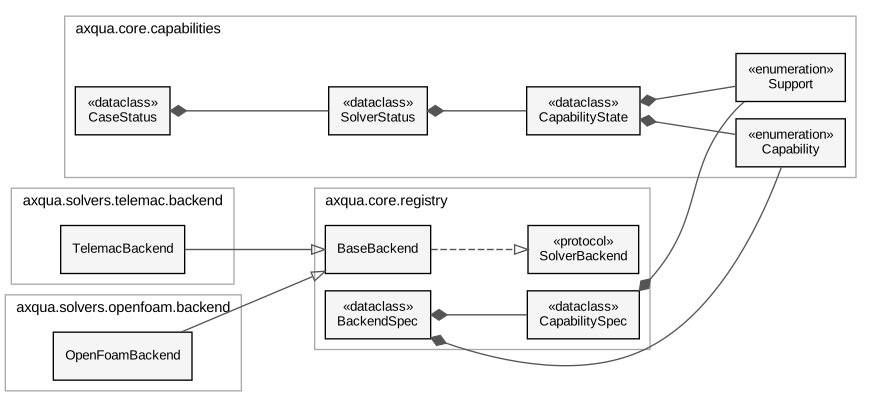
The simulation codes behind one interface. Both backends are derived from BaseBackend, which fulfills the interface SolverBackend. BackendSpec describes a backend and its capabilities without loading it.

What a case can do: the capability vocabulary and the MODEL= marker files.

A axqua case folder used to say nothing about itself. You could not tell, without reading the config and poking at axqua-case/, which solvers were set up, which features axqua actually implements for them, or how far this particular case had got. This module makes that explicit and writes it next to case-config.yml.

Three axes, deliberately kept apart

Conflating these is the mistake this module exists to avoid, because each answers a different user question and each has a different fix:

implemented

Does axqua support this capability for this solver at all? A static property of the code, from the backend’s own matrix. Three values, not two: OpenFOAM’s steady2d is not applicable (a VOF free-surface model is inherently 3D and transient), while its morphodynamics is not implemented (it could be; it isn’t yet). Telling a user “no” for both would be misleading - one is a gap in axqua, the other is a category error.

configured

Does this case ask for it? Derived from the config alone: a varying inflow series implies unsteady, morphodynamics.enabled implies GAIA, calibration parameters imply a BAL run.

built / run

Do the artifacts exist on disk? A pure path check per backend, so it stays cheap and never launches anything.

Why the files are generated and gitignored

The marker’s name (MODEL=TELEMAC_ENABLED) reflects the case - whether the config declares that solver - so it is portable and means the same on any machine. Its body reports this machine and this working tree: whether the solver environment resolves, and what has been built. That is local state, exactly like axqua-case/, so the files are regenerated rather than tracked; a tracked copy would churn on every build and would be a confident lie in a fresh clone. cases/case-template/ ships one committed example so the format stays documented.

Import weight

Standard library only, and it must stay that way. Enumerating what a case can do has to work in a process that has never imported gmsh, rasterio or OpenFOAM - a future QGIS plugin will do exactly that. Everything here works on paths and plain attribute access.

class axqua.core.capabilities.Capability(*values)

Bases: str, Enum

The shared vocabulary. One name per modeling capability, across all solvers.

Shared on purpose: “does this reach have an unsteady case” is the same question whichever code answers it, and a per-solver vocabulary would make the status table unreadable and the registry useless.

STEADY2D = 'steady2d'

UNSTEADY2D = 'unsteady2d'

STEADY3D = 'steady3d'

UNSTEADY3D = 'unsteady3d'

FREE_SURFACE_3D = 'free_surface_3d'

MORPHODYNAMICS = 'morphodynamics'

CALIBRATION = 'calibration'

MESH_CONVERGENCE = 'mesh_convergence'

VERTICAL_CONVERGENCE = 'vertical_convergence'

GAIN_LOSE = 'gain_lose'

class axqua.core.capabilities.Support(*values)

Bases: str, Enum

Whether a backend implements a capability, and if not, why not.

SUPPORTED = 'yes'

NOT_IMPLEMENTED = 'no'

NOT_APPLICABLE = 'n/a'

class axqua.core.capabilities.CapabilityState(capability, implemented, configured=None, built=None, run=None)

Bases: object

One capability’s state on all three axes for one solver.

Parameters:

• capability (Capability)

• implemented (Support)

• configured (bool | None)

• built (bool | None)

• run (bool | None)

capability: Capability

implemented: Support

configured: bool | None = None

built: bool | None = None

run: bool | None = None

property available: bool

implemented here and asked for by this case.

Type:

Ready to use

row()

Return type:

str

as_dict()

JSON form, for axqua case-status --json.

The three axes stay separate and the unknown ones stay null. A GUI needs that distinction: n/a means hide the tab (a category error for this solver), no means show it disabled with a reason (axqua has not built it yet), and null means “could not tell” - which is never the same as “no”.

Return type:

dict

class axqua.core.capabilities.SolverStatus(name, enabled, capabilities=<factory>, env_ok=None, env_detail='', case_name='', generated='', version='')

Bases: object

Everything the marker file records about one solver.

Parameters:

• name (str)

• enabled (bool)

• capabilities (list[CapabilityState])

• env_ok (bool | None)

• env_detail (str)

• case_name (str)

• generated (str)

• version (str)

name: str

enabled: bool

capabilities: list[CapabilityState]

env_ok: bool | None = None

env_detail: str = ''

case_name: str = ''

generated: str = ''

version: str = ''

property marker_name: str

capability(cap)

Parameters:

cap (Capability)

Return type:

CapabilityState | None

as_dict()

Return type:

dict

render()

The marker file body. Strictly parseable: # comments, key = value header, then a fixed-width table after [capabilities].

Return type:

str

write(case_dir)

Write the marker, removing any stale one for this solver first.

The removal matters: enabling a solver flips the filename, so without it a case would keep a contradictory MODEL=OPENFOAM_DISABLED beside its new MODEL=OPENFOAM_ENABLED.

Parameters:

case_dir (str | Path)

Return type:

Path

axqua.core.capabilities.read_marker(path)

Parse a marker file back into a SolverStatus.

Round-tripping is not decoration: it is the contract a QGIS plugin (or any other tool) reads, so it is tested rather than assumed.

Parameters:

path (str | Path)

Return type:

SolverStatus

class axqua.core.capabilities.CaseStatus(case_dir, solvers=<factory>, display=<factory>)

Bases: object

The whole case: one SolverStatus per registered backend.

Parameters:

• case_dir (Path)

• solvers (list[SolverStatus])

• display (dict)

case_dir: Path

solvers: list[SolverStatus]

display: dict

The case’s own display thresholds, for whoever draws its results. Carried here because the plugin asks this document what a case is, and these are properties of the REACH: hydrodynamics.wet_depth is the depth below which water is not surface flow (and is the threshold aXqua’s own reports already use, so a map drawn to a different one disagrees with its own report), and postproc.velocity_scale_max is the top of the velocity color scale, which a chute and a lowland river do not share.

classmethod collect(cfg, *, check_env=False)

Build the status for cfg from every registered backend.

check_env is off by default because probing an environment means spawning a shell per solver; the CLI turns it on, a bulk listing leaves it off.

Parameters:

check_env (bool)

Return type:

CaseStatus

solver(name)

Parameters:

name (str)

Return type:

SolverStatus | None

write_markers()

Return type:

list[Path]

as_dict()

The whole case as JSON. This is the plugin’s tab-generation contract.

The QGIS plugin builds its tab set from this rather than hardcoding one, so adding a capability - or a whole solver - to axqua surfaces in the plugin with no plugin change. It must stay standard-library-only for the same reason the rest of this module does: a plugin asking “what can this case do?” has to get an answer without importing gmsh.

Return type:

dict

render()

Return type:

str

write_and_summarise()

Return type:

list[str]

summary()

Short console form: one line per solver, then its available capabilities.

Return type:

list[str]

axqua.core.capabilities.refresh_markers(cfg)

Rewrite a case’s marker files. Never raises.

Called at the end of every build, so the files describe the case as it is now rather than as it was when someone last ran axqua status. A build that succeeded must not be reported as failed because a status file could not be written, hence the blanket catch.

Return type:

list[Path]

The solver registry: how axqua finds, describes and loads a simulation backend.

axqua used to reach for TELEMAC directly - pipeline.run imported steering, selafin and the rest by name, so adding a second code meant copying the pipeline rather than plugging into it. This module is the seam that replaces that.

Two objects, and the split between them is the whole design

BackendSpec

Metadata, and nothing else: the backend’s name, which capabilities it implements, which config block it owns, and where to find each of the capability-to-artifact path checks. Import-light by construction - a spec module may use the standard library and read attributes off a Config, and that is all.

SolverBackend

The implementation: build a case, run it, report on it. Loaded only when something actually needs to do work.

Keeping them apart is what lets axqua status - and, later, a QGIS plugin running inside the QGIS Python process - answer “what can this case do?” without importing gmsh, rasterio, or OpenFOAM’s Python. That question gets asked far more often than “now go and mesh it”, and it must stay cheap.

Adding a backend

Third-party backends are discovered through the axqua.solvers entry-point group, pointing at a module attribute that is a BackendSpec:

[project.entry-points."axqua.solvers"]
basement = "axqua_basement.spec:SPEC"

The built-ins register through the same mechanism, with a hard-coded fallback list so a source checkout that has not been re-installed still works. “Add your own” and “use ours” are therefore the same path, which is the only way the extension point stays honest.

class axqua.core.registry.CapabilitySpec(support, configured=None, built=None, run=None)

Bases: object

How to answer the three axes for one capability, without running anything.

Parameters:

• support (Support)

• configured (Callable[[object], bool] | None)

• built (Callable[[object], bool] | None)

• run (Callable[[object], bool] | None)

support: Support

configured: Callable[[object], bool] | None = None

built: Callable[[object], bool] | None = None

run: Callable[[object], bool] | None = None

evaluate(capability, cfg)

Fill in the axes that apply. Anything the backend cannot answer is left None and renders as - rather than as a confident no.

Parameters:

capability (Capability)

Return type:

CapabilityState

class axqua.core.registry.BackendSpec(name, title, config_key, capabilities=<factory>, implementation='', enabled=None, environment=None)

Bases: object

Import-light description of a solver backend.

Parameters:

• name (str)

• title (str)

• config_key (str)

• capabilities (Mapping[Capability, CapabilitySpec])

• implementation (str)

• enabled (Callable[[object], bool] | None)

• environment (Callable[[object], str] | None)

name: str

title: str

config_key: str

capabilities: Mapping[Capability, CapabilitySpec]

implementation: str = ''

enabled: Callable[[object], bool] | None = None

environment: Callable[[object], str] | None = None

support(capability)

Parameters:

capability (Capability)

Return type:

Support

is_enabled(cfg)

Return type:

bool

status(cfg, *, check_env=False)

Evaluate every capability for cfg.

Parameters:

check_env (bool)

Return type:

SolverStatus

check_environment(cfg)

Whether this machine can actually run the solver.

Probes the configured environment (axqua.core.environment) and checks it yields that solver’s sentinel variables - so a wrong setup script is caught here rather than hours into a job. Only ever called when a caller asks for it (axqua status --check-env), because it spawns a shell.

Return type:

bool | None

load()

Import and return the implementation. The only heavyweight call here.

Return type:

SolverBackend

class axqua.core.registry.SolverBackend(*args, **kwargs)

Bases: Protocol

What an implementation must provide to be driven by axqua.

Intentionally small. Everything a backend needs that is not solver-specific - the geodata, the boundary conditions, the ground truth, the convergence maths - comes from axqua.core, so a new backend implements the parts that are genuinely its own and inherits the rest.

name: str

check_environment(cfg)

Can this machine run the solver? Must not raise.

Return type:

bool

build(cfg, capability, **kwargs)

Assemble the case for capability; return the produced artifacts.

Parameters:

capability (Capability)

run(cfg, capability, **kwargs)

Launch the solver on an already-built case.

Parameters:

capability (Capability)

study(cfg, capability, **kwargs)

Run a multi-run investigation: convergence ladder, calibration campaign.

A third verb rather than folding these into run(), because a study is genuinely neither a build nor a run - it repeatedly does both, decides when to stop, and reports on the sequence. Folding it into run would make every caller inspect the capability to know what it just started.

Parameters:

capability (Capability)

postprocess(cfg, ctx)

Turn raw solver output into results: reconstruction, reports, conversions.

Part of the runner lifecycle, deliberately (plan §13): QGIS must never do heavy OpenFOAM postprocessing, so the expensive step happens where the solver ran, before the job reports COMPLETED.

extract_objective(cfg, ctx)

The single number a calibration is minimizing, if this job produced one.

Return type:

float | None

export_qgis_results(cfg, ctx)

Write results/qgis/ and describe it in the result manifest.

Never imports PyQGIS. It creates files and says what they are; the plugin loads and styles them (plan §14). That separation is what lets the runner work on a headless cluster node.

describe_results(cfg)

What a visualizer can open for this case, in solver-neutral terms.

The counterpart to export_qgis_results(): that one writes files for QGIS, this one describes what already exists so a post-processing backend (axqua.postproc) can draw it without knowing which solver produced it. Returns axqua.postproc.dataset.Dataset values.

This is the seam that keeps postproc from importing a solver: the knowledge of where a result lives and what fields and patches it carries is the backend’s, and it is handed over as data. Returning [] means “nothing to draw yet”, never an error.

Return type:

list

class axqua.core.registry.BaseBackend

Bases: object

Optional base supplying no-op defaults for the parts a backend does not have.

SolverBackend has six methods, and a third-party backend that only builds cases should not have to write four stubs to satisfy a runtime_checkable protocol. Subclassing is not required - the protocol is structural - but it removes the boilerplate and documents which parts are genuinely optional.

name: str = ''

check_environment(cfg)

Return type:

bool

build(cfg, capability, **kwargs)

Parameters:

capability (Capability)

run(cfg, capability, **kwargs)

Parameters:

capability (Capability)

study(cfg, capability, **kwargs)

Parameters:

capability (Capability)

postprocess(cfg, ctx)

extract_objective(cfg, ctx)

Return type:

float | None

export_qgis_results(cfg, ctx)

describe_results(cfg)

Return type:

list

axqua.core.registry.register(spec, *, replace=False)

Add spec to the registry (idempotent unless replace).

Parameters:

• spec (BackendSpec)

• replace (bool)

Return type:

BackendSpec

axqua.core.registry.discover(*, force=False)

Populate the registry from the built-ins and the entry-point group.

Parameters:

force (bool)

Return type:

None

axqua.core.registry.backends()

Every registered backend spec, in registration order.

Return type:

list[BackendSpec]

axqua.core.registry.get(name)

One backend spec by name.

Parameters:

name (str)

Return type:

BackendSpec

axqua.core.registry.names()

Return type:

list[str]

axqua.core.registry.supporting(capability)

Backends that implement capability - the “which code can do this?” query.

Parameters:

capability (Capability)

Return type:

list[BackendSpec]